The Principle of Least Action and the Euler-Lagrange Equation

In physics, this “laziness” is elegantly described by the Principle of Least Action. Instead of calculating the forces acting on an object at every instant (as in Newtonian mechanics), we look at the path as a whole and ask: which trajectory spends the smallest amount of “Action”?

“The mathematics of laziness”

To understand this mathematically, we need to introduce the Lagrangian ($L$). The Lagrangian is simply the difference between Kinetic Energy ($T$, the energy of motion) and Potential Energy ($V$, stored energy).

$$L = T - V$$

The “Action” ($S$) is the integral of the Lagrangian over the time during which the object is moving, expressed by the integral:

$$S = \int^{t1}_{t2} L dt$$

The Principle of Least Action states that the actual trajectory an object follows between two points is the one that makes the Action ($S$) minimal. To find this path, we use the Euler-Lagrange equation:

$$\frac{d}{dt} \left( \frac{\partial L}{\partial \dot{q}} \right) - \frac{\partial L}{\partial q} = 0$$

• $q$ represents position
• $\dot{q}$ represents velocity (the derivative of position).

When we solve this equation, we find the exact trajectory that nature chooses.

Translating Physics into Code

Explaining the theory is nice, but proving it in code brings the idea into the real world. Since a computer doesn’t solve differential equations analytically the way a human does on paper, we can turn the Principle of Least Action into a computational optimization problem.

We can define a starting point and an ending point, create random paths between them, and ask an algorithm to compute the Action of all of them. The algorithm will adjust the path until it finds the smallest possible value.

Here is how we can simulate the trajectory of an object in free fall using numerical optimization:

import numpy as np
from scipy.optimize import minimize
import matplotlib.pyplot as plt

# Problem parameters
m = 1.0
g = 9.81
t_start = 0
t_end = 2.0
N = 20

# Time vector and time step (dt)
t = np.linspace(t_start, t_end, N)
dt = t[1] - t[0]

# The Action function
def compute_action(y):
  # Velocity is the difference in position over time
  v = (y[1:] - y[:-1]) / dt
  # Kinetic Energy (T = 0.5 * m * v^2)
  T = 0.5 * m * np.sum(v**2)
  # Potential Energy (V = m * g * y)
  V = m * g * np.sum(y[:-1])
  # Action S = Integral of (T - V) dt
  L = T - V
  action = L * dt
  return action

# Initial guess: a straight line from point A to point B
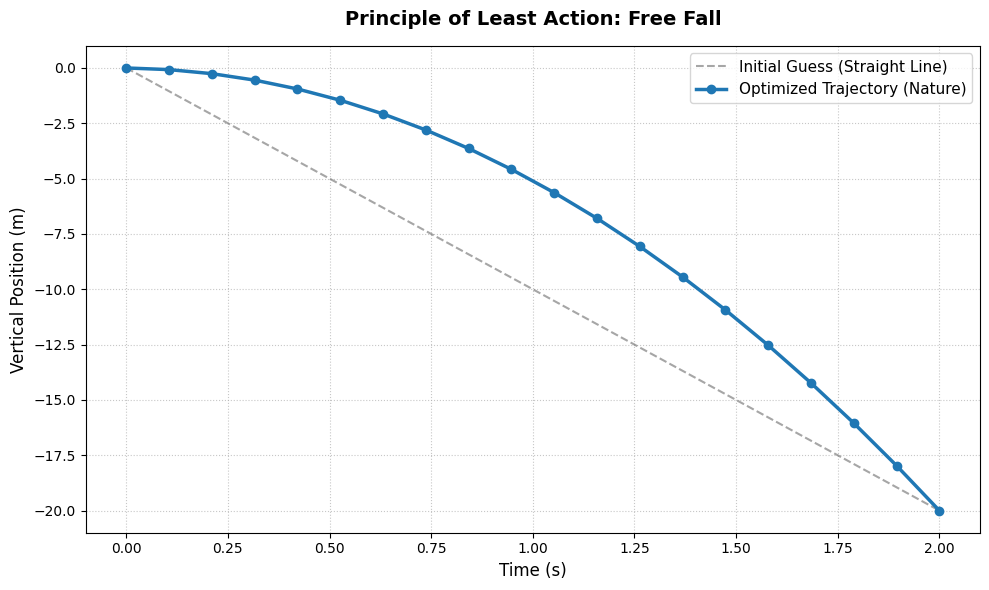
y_initial = np.linspace(0, -20, N)
# We need to lock the first and last points (they can't change)
# y[0] = 0 (start) and y[-1] = -20 (end)
constraints = [
    {'type': 'eq', 'fun': lambda y: y[0] - 0},
    {'type': 'eq', 'fun': lambda y: y[-1] - (-20)}
]

result = minimize(compute_action, y_initial, constraints=constraints)
optimized_path = result.x

print("Path found by nature:", optimized_path)

What happens behind the scenes of the code?

1. Defining the Rule: The compute_action function calculates kinetic energy minus potential energy for any possible path we feed into it.
2. Imposing Constraints: The constraints tell the computer: “The object MUST start at point A and end at point B. What happens in between is up to you.”
3. The Optimization: The minimize function (from the SciPy library) acts as nature itself. It tries small variations on the intermediate points (y_initial). If a change decreases the total Action, it keeps it; if it increases it, it discards it (this is how a computer solves a derivative).

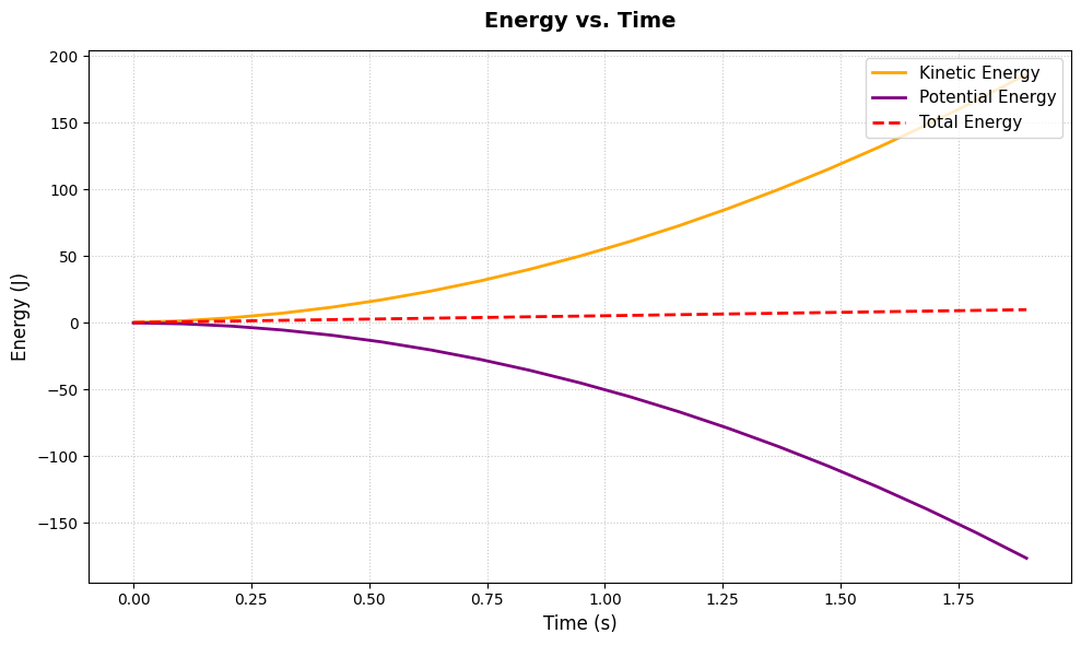
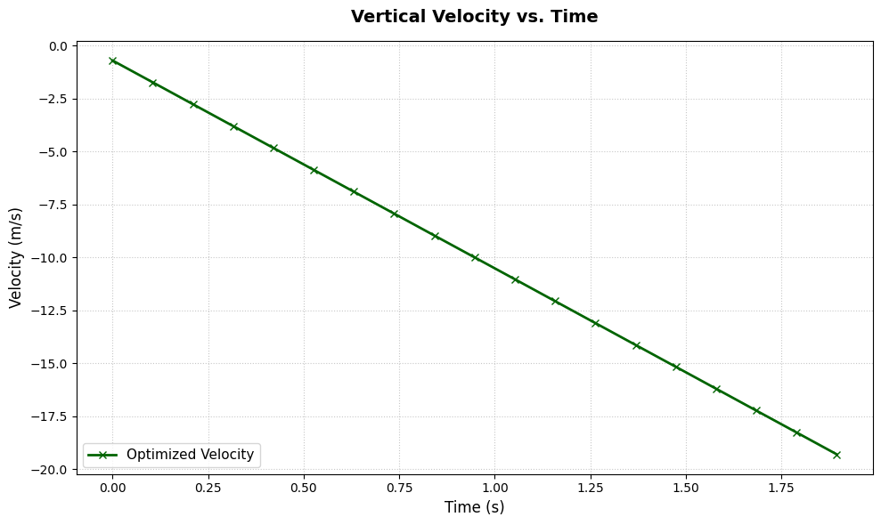
At the end of the optimization loop, the computer draws exactly a perfect mathematical parabola, as can be seen in the image below. Without using any Newtonian force in the code, the computer “discovers” gravity simply by being instructed to spend the smallest amount of energy possible.

Where Do We Go Now? From Physics to the Real World of Computing

The Euler-Lagrange equation and the Principle of Least Action may seem, at first glance, like tools exclusive to physicists calculating the trajectories of planets or particles. However, the heart of this mathematical idea — finding the optimal path by minimizing a variable — is the invisible engine of almost all modern technology.

In nature, we minimize the “Action”. In computing, we minimize the “Cost”.

How does this principle work in everyday life?

1. The Heart of Artificial Intelligence (Machine Learning) If you’ve ever used modern AI tools, code assistants, or text generators, know that they operate under a logic almost identical to that of nature. During the training of a model, the AI doesn’t know the right answer right away. Instead, it has a Loss Function — an equation that measures how “wrong” the AI is. Using optimization algorithms (like Gradient Descent), the AI adjusts its parameters step by step to find the point where the error is as small as possible. It’s the Principle of Least Action applied to the mathematics of data.

2. Back-End Programming and System Optimization When we build complex systems (whether using Python, C#, or microservice architectures), we constantly deal with routing algorithms and resource allocation. Pathfinding algorithms (like the famous Dijkstra or A*) look for the shortest route in a network graph to save latency and processing. The system is programmed to be as “lazy” as nature: delivering data from point A to point B spending the smallest amount of memory and CPU time possible.